連続な関数f(θ, φ)の球面調和関数展開
球面調和関数の係数を求めるには、$c_{l}^{m} = <f, Y_{l}^{m}>$として内積を取る。数学的にはこれで終わりだが、現実に係数を得るには積分計算のところを数値計算する必要がある。
適当な関数で試してみる。scipy.integrate.dblquadは、dblquad(func, a, b, gfun, hfun)で、$\int_{a}^{b}dx \int_{ \text{gfun(x)} }^{ \text{hfun(x)} }dy \text{func}(y, x)$という二重積分を表す。返り値は(積分値、誤差)のタプルになっている。yとxの順番が気に入らないので書き換えてしまう
from scipy.integrate import dblquad as _dblquad
def dblquad(func, mx, Mx, my, My):
    return _dblquad(lambda x, y: func(y, x), mx, Mx, lambda x: my, lambda x: My)
import numpy as np
from scipy.special import sph_harm as _sph_harm
from scipy.integrate import dblquad as _dblquad
from mpl_toolkits.mplot3d import Axes3D
import matplotlib.pyplot as plt
import matplotlib.cm as cm

# user modification
def sph_harm(l, m, theta, phi):
    if m > 0:
        return np.sqrt(2) * (-1)**m * _sph_harm(m, l, phi, theta).real
    if m == 0:
        return _sph_harm(m, l, phi, theta).real
    else:
        return np.sqrt(2) * (-1)**m * _sph_harm(-m, l, phi, theta).imag
def dblquad(func, mx, Mx, my, My):
    return _dblquad(lambda x, y: func(y, x), mx, Mx, lambda x: my, lambda x: My)

# 展開
def f(u, v):
#    return 1
#    return np.cos(u)
#    return 1 + np.sin(v)**2
    return (2 + np.sin(2 * v)) * (2 + np.sin(u))

# 内積
def inner(func, l, m):
    I = lambda u, v: func(u, v) * sph_harm(l, m, u, v) * np.sin(u)
    return dblquad( I, 0, np.pi, 0, 2 * np.pi )[0]

Lmax = 20
c = []
for l in range(Lmax + 1):
    for m in range(-l, l+1):
        # append c_lm to c
        c.append( inner(f, l, m) )

fig = plt.figure()

# 展開前
ax = fig.add_subplot(411, projection="3d")

u = np.linspace(0, np.pi, 100)
v = np.linspace(0, 2 * np.pi, 100)
r0 = np.array([[f(_u, _v) for _v in v] for _u in u])

x0 = r0 * np.outer(np.sin(u), np.cos(v))
y0 = r0 * np.outer(np.sin(u), np.sin(v))
z0 = r0 * np.outer(np.cos(u), np.ones(v.size))

surf = ax.plot_surface(x0, y0, z0, color='r',
        rstride=2, cstride=2, linewidth=1, shade=False)

# 展開後
r = np.zeros([u.size, v.size])
diff_r = []
pos = 2

for l in range(Lmax+1):
    for m in range(-l, l+1):
        # 球面調和関数を足し合わせる
        r += c[l**2 + l + m] * sph_harm(l, m, np.array(u, ndmin=2).T, v)
        diff_r.append( ((r - r0)**2).sum() )

    if (l in (0, 5, 20)):
        ax = fig.add_subplot(4,1,pos, projection="3d")
        pos += 1

        x = r * np.outer(np.sin(u), np.cos(v))
        y = r * np.outer(np.sin(u), np.sin(v))
        z = r * np.outer(np.cos(u), np.ones(v.size))

        surf = ax.plot_surface(x, y, z, color='b',
            rstride=1, cstride=1, linewidth=1, shade=False)

plt.show()
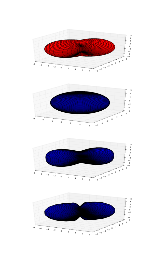
青が元の形状で赤は上から順にl=0,5,20の時の展開結果。次第に誤差が少なくなっているように見える。
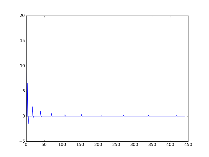
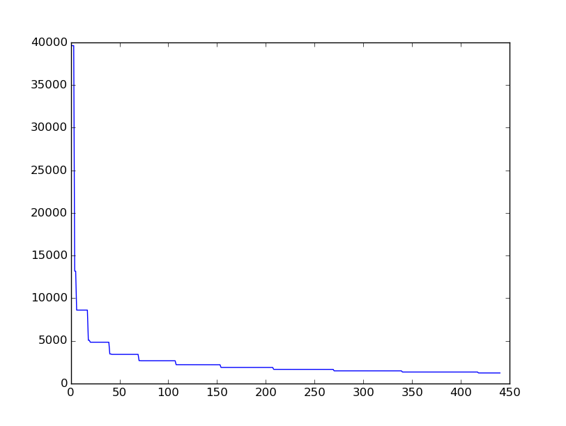
左が係数、右が元の座標との2乗誤差の変化を表す。係数が次第に0に近づいていること、誤差が0に向かって小さくなっていることが分かる。